Data from a longitudinal study of adolescents in the state of Victoria carried out between August 1992 and July 1995. Approximately 2,000 adolescents were recruited and followed up at six timepoints (“waves”) at six-monthly intervals. Some of the participants were not recruited until the second wave
We will focus on one of the smoking measures: regular smoking. Smoking behaviour was determined at each wave using a 7-day retrospective diary, completed by all participants except those who considered themselves non-smokers or ex-smokers (no cigarette in the previous month). From the diary response, a subject was categorized as a “regular smoker” if they reported smoking on at least six days of the previous week.
We are interested in determining the prevalence of smoking for each gender and investigating how this changes with age. Secondary questions concern the association between the prevalence of smoking and baseline factors such as parental smoking.
Variable name
Description
id
Participant identifier
age
Age of participant at survey wave (years)
wave
Wave of data collection (1,2,…,6)
sex
Sex (0=male, 1=female)
parsmk
Parental smoking (1=at least one parent smokes most days, 0=otherwise)
regsmoke
Regular smoker (1=participant reports smoking at least 6 days a week, 0=otherwise)
      id school wave      age  sex born_oz parsmk regsmoke   wgt_mv wgt_str
1 920006   3010    1 14.17488 male       1      0        0 2.142857 0.77829
2 920006   3010    2 14.73357 male       1      0        0 1.120879 0.77829
3 920006   3010    3 15.17214 male       1      0        0 1.115974 0.77829
4 920006   3010    4 15.65571 male       1      0        0 1.183295 0.77829
5 920006   3010    5 16.12012 male       1      0        0 1.217184 0.77829
6 920006   3010    6 16.67762 male       1      0        0 1.256158 0.77829
  sregion
1     InU
2     InU
3     InU
4     InU
5     InU
6     InU
Label sex variable
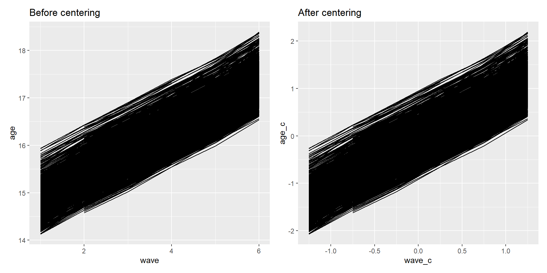
Before analysis, we should center variables by subtracting the sample mean from each observation because:
It makes the intercept more interpretable by creating a meaningful zero point; when the coefficient is negative, it is below the population mean, and when the coefficient is positive, it is above the population mean.
## centering age and wave variablessmoke_prev <-transform(smoke_prev, age_c = age -16.2,wave_c = (wave -3.5)/2)
Abbreviations: CI = Confidence Interval, OR = Odds Ratio
Intercept: the odds of being a regular smoker for the reference group (males) at the reference value of age (age_c = 0)
sex: Difference in odds of regular smoking between males and females at age_c = 0
Coefficient at (third line): Change in odds of regular smoking per 1-unit increase in age (centered) among males
Coefficient at (fourth line): Change in odds of regular smoking per 1-unit increase in age (centered) among females
4.4 Incorporate correlation in outcome data: GEE
Unlike the normal distribution, binomial has no natural multivariate version, so full probability model approach to logistic regression is more challenging
However, as previously with continuous outcome, the generalized estimating equations produce unbiased coefficient estimates under certain conditions
Specify working correlation matrix and use robust variance estimates
library(geepack); library(gee)robglm.fit1 <-geeglm(regsmoke ~ sex*age_c, data = smoke_prev, family =binomial,id=id)summary(robglm.fit1)
Abbreviations: CI = Confidence Interval, OR = Odds Ratio
Note
As shown, the coefficient estimates are identical, but the 95% confidence interval is wider and the p-value is larger for the sex coefficient compared with the standard logistic regression. By using robust variance estimation, GEE accounts for potential within-individual correlation and answers the question, “If observations within an individual are correlated, how uncertain should the estimates be?” These results suggest reduced effective information for time-invariant covariates.