2  Generalized Estimating Equation

2.1 Data description

Potthoff and Roy growth data:

• Growth measurements for 27 children (11 girls and 16 boys)

• Distance (in mm) from the centre of the pituitary gland to the pterygo-maxillary fissure recorded at ages 8, 10, 12 and 14 years.

• Interested in the differences between males and females in pattern of growth over the 4 time points (from age 8 to 14 years).

library(haven)
library(ggplot2)
library(dplyr)
library(tidyr)
library(stringr)
library(mice)
library(ggcorrplot)
library(gtsummary)

potthoffroy |> 
  pivot_longer(cols = -c(id,sex)) |> 
  mutate(age = str_extract(name,'\\d+') |> as.numeric()) |> 
  ggplot(aes(x = age,y = value))+
  geom_line(aes(group = id))+
  facet_wrap(~sex)+
  theme_bw()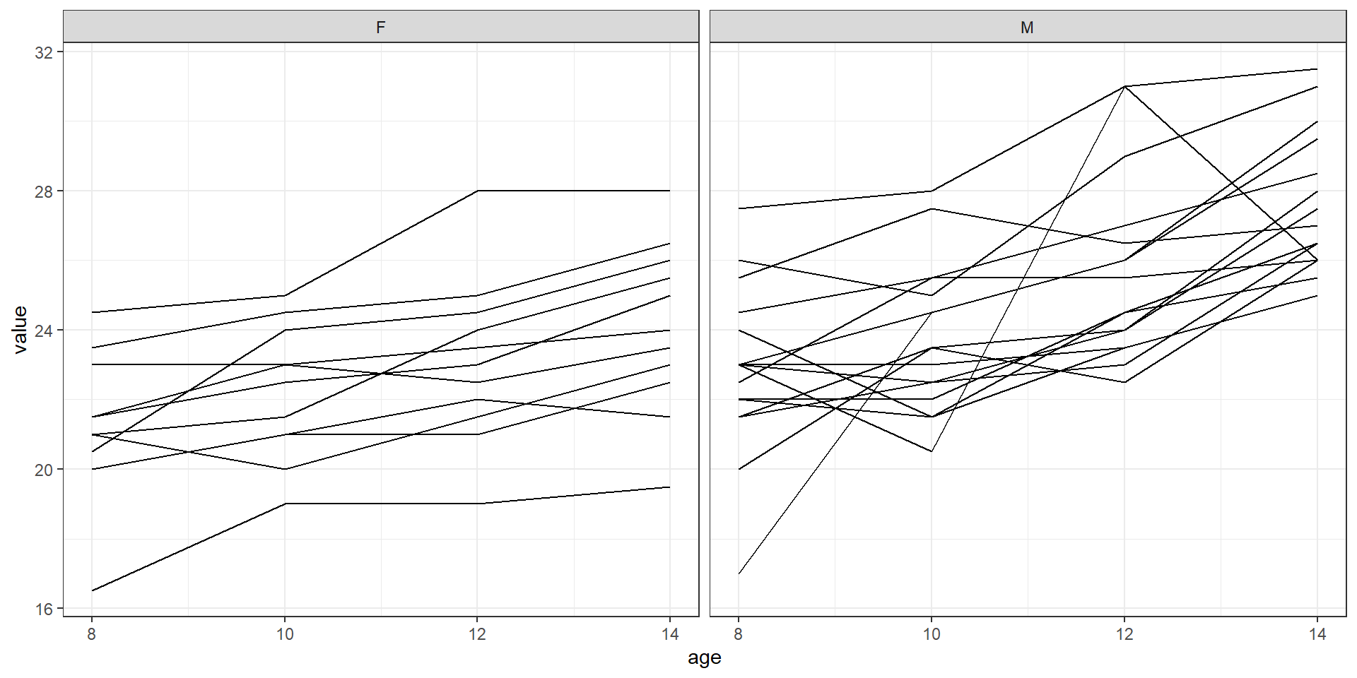

We consider the correlation of the value in male and female group

potthoffroy |> 
  filter(sex == "M") |> 
  select(-c(id,sex)) |> 
  cor(use="pairwise.complete.obs")|> 
  ggcorrplot(lab = TRUE) +
  labs(tag = "Male")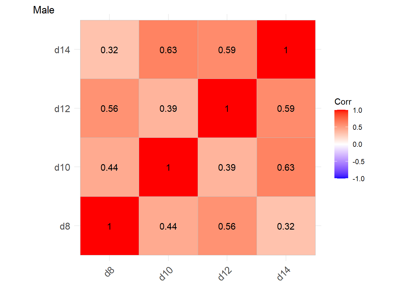

potthoffroy |> 
  filter(sex == "F") |> 
  select(-c(id,sex)) |> 
  cor(use="pairwise.complete.obs")|> 
  ggcorrplot(lab = TRUE) +
  labs(tag = "Female")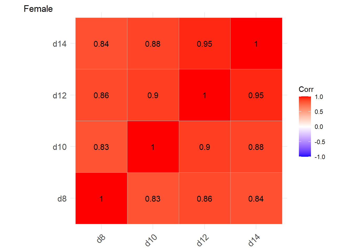

NoteConclusion

Positive correlations within-cluster. Greater for Females than Males.

2.2 Fitting OLS

data <- potthoffroy |> 
  pivot_longer(cols = -c(id,sex)) |> 
  mutate(age = str_extract(name,'\\d+') |> as.numeric(),
         sex = factor(sex,labels = c(0,1))) 

lm_model <- lm(value ~ sex + age, data = data)

summary(lm_model)

Call:
lm(formula = value ~ sex + age, data = data)

Residuals:
    Min      1Q  Median      3Q     Max 
-5.9882 -1.4882 -0.0586  1.1916  5.3711 

Coefficients:
            Estimate Std. Error t value Pr(>|t|)    
(Intercept) 15.38569    1.12857  13.633  < 2e-16 ***
sex1         2.32102    0.44489   5.217 9.20e-07 ***
age          0.66019    0.09776   6.753 8.25e-10 ***
---
Signif. codes:  0 '***' 0.001 '**' 0.01 '*' 0.05 '.' 0.1 ' ' 1

Residual standard error: 2.272 on 105 degrees of freedom
Multiple R-squared:  0.4095,    Adjusted R-squared:  0.3983 
F-statistic: 36.41 on 2 and 105 DF,  p-value: 9.726e-13

Warning

Pretend observations independent – WRONG!!

The estimation of beta (sex, age, intercept) is unbiased, but the standard errors are incorrect if the covariance is not independent.

Note

• \(\widehat{\beta}\) are estimated using Odinary Least Square

• \(Var(\widehat{\beta})\) - derived from covariance matrix of \(Y\), known as V

  Covariance = variance \(\times\) correlation

  Conventional regression model fit by OLS has \(V_i = \sigma^2I_{n_i \times n_i}\)

2.3 How can we estimate the correct variance of the OLS estimator when the data are not independent?

Robust / empirical / “sandwich” variance estimator:

• Use actual correlations observed in the data (i.e. empirical correlations)

• Robust – for a large number of clusters it converges to the correct variance of the OLS parameter estimate, irrespective of what the true covariance V is, as long as the corrected model for the mean of Y has been specified.

• Sandwich: the data driven empirical estimator is the “meat” in the sandwich between two model-based terms (“slices of bread”)

library(lmtest)
library(sandwich)

lm_model <- lm(value ~ sex + age, data = data)

## Robust step
cov_cl <- vcovCL(lm_model, cluster = data$id)
cov_cl

            (Intercept)       sex1          age
(Intercept)  0.87447024 -0.3160789 -0.050590613
sex1        -0.31607886  0.5948969 -0.006492700
age         -0.05059061 -0.0064927  0.005173734

se_robust_model <- coeftest(lm_model, vcov = cov_cl)

se_robust_model

t test of coefficients:

             Estimate Std. Error t value  Pr(>|t|)    
(Intercept) 15.385690   0.935131 16.4530 < 2.2e-16 ***
sex1         2.321023   0.771296  3.0093  0.003279 ** 
age          0.660185   0.071929  9.1783 4.268e-15 ***
---
Signif. codes:  0 '***' 0.001 '**' 0.01 '*' 0.05 '.' 0.1 ' ' 1

Compare

lm_model |> 
tbl_regression(
  intercept = TRUE,
  estimate_fun = purrr::partial(style_ratio, digits = 3)) |> 
  remove_row_type(
    type = "reference"
  )

Characteristic	Beta	95% CI	p-value
(Intercept)	15.39	13.15, 17.62	<0.001
sex
1	2.321	1.439, 3.203	<0.001
age	0.660	0.466, 0.854	<0.001
Abbreviation: CI = Confidence Interval

se_robust_model |> 
  tbl_regression(
    intercept = TRUE,
    estimate_fun = purrr::partial(style_ratio, digits = 3)
  ) 

Characteristic	Beta	95% CI	p-value
(Intercept)	15.39	13.53, 17.24	<0.001
sex1	2.321	0.792, 3.850	0.003
age	0.660	0.518, 0.803	<0.001
Abbreviation: CI = Confidence Interval

Sex: difference in mean outcome between sexes at any age = between-subject comparison

• SE with robust > SE assuming independence (0.7712956 > 0.4448862)

• Between cluster comparison is LESS precise with positive within-subject correlation

Age: effect estimated within-subject.

• SE with robust < SE independence ( 0.0719287 < 0.0977589)

• Within-cluster comparison is MORE precise with positive correlation

NoteConclusion

As we can see, within-cluster comparison is MORE precise with positive correlation. By modelling the covariance V correctly using the robust variance estimator instead of assuming independence, we generally obtain smaller standard errors. How to model covariance V?

2.4 Common correlation / covariance structures

1. Exchangeable: correlation between any two measurements on an individual is the same no matter how far apart in time they are.

2. Autoregressive: correlation decreases with distance

3. Unstructured: no pre-determined structure

Putting together in GEE

The covariance V is unknown, but take a “guest” at its form.

Call this W (e.g. exchangeable, autoregressive, etc.)

• Can get idea from empirical correlations

• Called a “working” covariance – we know it may be wrong but we work with it anyway

Step for GEE:

1. Fit OLS regression, and estimate parameters in W using residuals from OLS regression

2. Solve weighted least squares regression using \(\widehat{W}\) to get \(\widehat{\beta}_W\)

3. Iterate between \(\widehat{W}\) and \(\widehat{\beta}_W\) until convergence

2.5 Example data

Data from a study investigating recovery following appendectomy in children. The aim of the study was to determine whether the children who underwent a laparoscopic appendectomy achieved a faster rate of recovery than children who underwent conventional “open” appendectomy.

In this study a measure of recovery was made using an “uptimer”, a device worn by the children on their thigh. The uptimer senses the position of the thigh and records the times of changes from a horizontal position to a “vertical” position (at least 45 degrees from the horizontal). An increasing number of position changes (horizontal to vertical) from one day to the next is a marker of recovery.

appendix <- read_dta("./data/appendix.dta")

appendix <- appendix |> 
  mutate(lognchanges = log(nchanges),
         group = factor(group,labels = c("Lap","Open")))  

Plot the distribution of number of change

appendix |> 
  ggplot(aes(nchanges))+
  geom_histogram()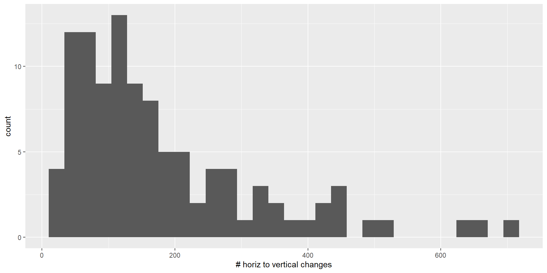

This seem like a skewed distribution, so we will use logarithm

appendix |> 
  ggplot(aes(lognchanges))+
  geom_histogram()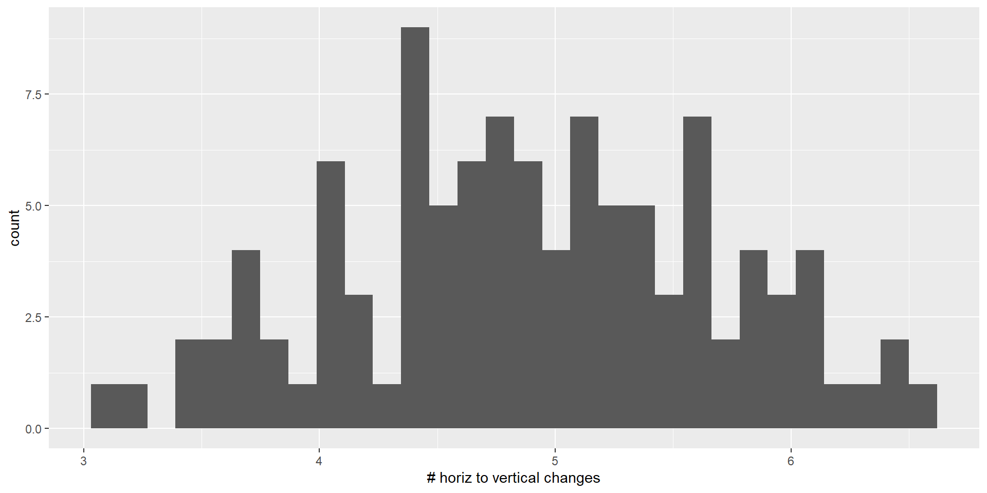

And we will see the description of the data

appendix |> 
  ggplot(aes(x = day, y = lognchanges))+
  geom_line(aes(group = patid))+
  geom_point()+
  facet_wrap(~group)+
  theme_bw()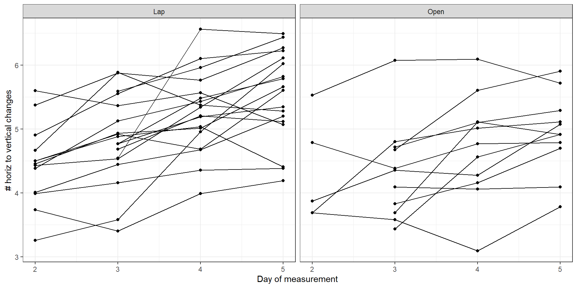

Using GEE with different working covariance \(W\)

The research question is whether the rate of change of the outcome variable – logged number of position changes – differs between the two groups. In order to address this within a regression modeling framework, we need to model the relationship between the outcome and time, and allow this relationship to differ between groups. The effect of surgical group will then be measured by a single interaction parameter.

library(geepack); library(gee)

Independence

geefit.ind <- geeglm(lognchanges~day*group,
                     data = appendix,  
                     id = patid, 
                     corstr = "independence")
summary(geefit.ind)

Call:
geeglm(formula = lognchanges ~ day * group, data = appendix, 
    id = patid, corstr = "independence")

 Coefficients:
              Estimate  Std.err    Wald Pr(>|W|)    
(Intercept)    3.74588  0.29367 162.700  < 2e-16 ***
day            0.36338  0.07159  25.763 3.86e-07 ***
groupOpen     -0.04868  0.50811   0.009    0.924    
day:groupOpen -0.11807  0.11090   1.133    0.287    
---
Signif. codes:  0 '***' 0.001 '**' 0.01 '*' 0.05 '.' 0.1 ' ' 1

Correlation structure = independence 
Estimated Scale Parameters:

            Estimate Std.err
(Intercept)   0.4488 0.08769
Number of clusters:   29  Maximum cluster size: 4 

Exchangeable

geefit.ex <- geeglm(lognchanges~day*group,
                      data = appendix, 
                      id = patid, 
                      corstr = "exchangeable")
summary(geefit.ex)

Call:
geeglm(formula = lognchanges ~ day * group, data = appendix, 
    id = patid, corstr = "exchangeable")

 Coefficients:
              Estimate Std.err   Wald Pr(>|W|)    
(Intercept)     3.8441  0.2724 199.13  < 2e-16 ***
day             0.3407  0.0676  25.41  4.6e-07 ***
groupOpen      -0.2163  0.4333   0.25     0.62    
day:groupOpen  -0.0794  0.1007   0.62     0.43    
---
Signif. codes:  0 '***' 0.001 '**' 0.01 '*' 0.05 '.' 0.1 ' ' 1

Correlation structure = exchangeable 
Estimated Scale Parameters:

            Estimate Std.err
(Intercept)    0.449   0.088
  Link = identity 

Estimated Correlation Parameters:
      Estimate Std.err
alpha    0.668  0.0988
Number of clusters:   29  Maximum cluster size: 4 

Autoregressive

geefit.ar1 <- geeglm(lognchanges~day*group,
                      data = appendix, 
                      id = patid, 
                      corstr = "ar1",wave=day)
summary(geefit.ar1)

Call:
geeglm(formula = lognchanges ~ day * group, data = appendix, 
    id = patid, waves = day, corstr = "ar1")

 Coefficients:
              Estimate Std.err   Wald Pr(>|W|)    
(Intercept)     3.7648  0.2494 227.89  < 2e-16 ***
day             0.3539  0.0656  29.12  6.8e-08 ***
groupOpen      -0.2869  0.4374   0.43     0.51    
day:groupOpen  -0.0613  0.1015   0.36     0.55    
---
Signif. codes:  0 '***' 0.001 '**' 0.01 '*' 0.05 '.' 0.1 ' ' 1

Correlation structure = ar1 
Estimated Scale Parameters:

            Estimate Std.err
(Intercept)     0.45  0.0882
  Link = identity 

Estimated Correlation Parameters:
      Estimate Std.err
alpha     0.76   0.079
Number of clusters:   29  Maximum cluster size: 4 

	Independence	Exchangeable	Auto-regressive 1
Group effect (on slope)	-0.1181	-0.0794	-0.0613
Robust SE of group effect (on slope)	0.1109	0.1007	0.1015