7  Hierachical ascending classification

7.1 Principle

7.1.1 First strategy: Agglomerative Hierarchical Clustering

• Start from the bottom of the dendrogram (singletons),

• Add the closest parts two by two until you get a single class

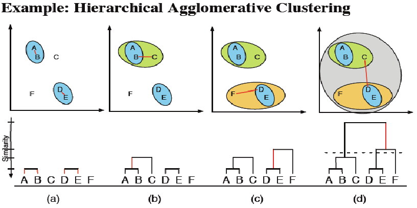
Source: @janssen2012

Source: Data analysis MOOC of Francois Husson

NoteWhere to cut the dendogram?

Rule of thumb

• Selection of a cut when there is a significant jump in the index by visual inspection of the tree. This jump reflects the sudden passage from a certain homogeneity of classes to much less homogeneous classes.

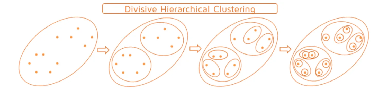
7.1.2 Second strategy: Divide the hierarchical clustering

• Start from the top of the dendrogram (one unique class),

• Successive divisions until you get classes reduced to singlets.

7.2 Weaknesses and strengths

Advantages

• Simple considerations of distances and similarities

• No assumption on the number of classes

• Can correspond to significant taxonomies

Disadvantages

• Choice of the dendogram cutoff.

• The partition obtained at a step depends on that of the previous step.

• Once a decision is made to combine classes, it cannot be undone.

• Too slow for large datasets.

7.3 Practical

7.3.1 Example 1

We consider the following data table where 4 individuals (here points) A,B,C and D are described on two variables (X1 and X2):

	X1	X2
A	5	4
B	4	5
C	1	-2
D	0	-3

7.3.1.1 Construct the dendrogram using maximal link

\(\mathcal{P}^{\{0\}} = \{\{A\},\{B\},\{C\},\{D\}\}\)

• Step 1:

\(d(A,B)\) = 1.4142136

\(d(A,C)\) = 7.2111026

\(d(A,D)\) = 8.6023253

\(d(B,C)\) = 7.6157731

\(d(B,D)\) = 8.9442719

\(d(C,D)\) = 1.4142136

	A	B	C	D
A	0
B	1.4142136	0
C	7.2111026	7.6157731	0
D	8.6023253	8.9442719	1.4142136	0

=> \(\mathcal{P}^{\{1\}} = \{\{A,B\},\{C\},\{D\}\}\)

We can choose: minimal link, maximum link, average link, or Ward’s link. In this case, I selected maximum link:

\[\begin{align} D(C_k,C_{k'}) = \max_{x \in C_k ,\: x' \in C_{k'}} d(x,x') \end{align}\]

• Step 2:

\(D(\{A,B\},\{C\}) \\\)

= \(max(d(A,C),d(B,C))\)

= \(max(7.21,7.61) = {\bf 7.61}\)

\(D(\{A,B\},\{D\}) \\\)

= \(max(d(A,D),d(B,D))\)

= \(max(8.6,8.9) = {\bf 8.9}\)

\(D(\{C\},\{D\}) = d(C,D) = 1.41\)

\(D(\{A\},\{B\}) = d(A,B) = 1.41\)

=> \(\mathcal{P}^{\{2\}} = \{\{A,B\},\{C,D\}\}\)

• Step 3:

\(D(\{A,B\},\{C,D\})\)

= \(max(d(A,C),d(A,D),d(B,C),d(B,D))\)

= 8.9

=> \(\mathcal{P}^{\{3\}} = \{A,B,C,D\}\)

d <- stats::dist(X) # compute the Euclidean distances between points

treeC <- hclust(d, method="complete")

treeC$height

[1] 1.414214 1.414214 8.944272

ggdendrogram(treeC, rotate = FALSE, size = 2)+
  scale_y_continuous(breaks = seq(0,10.5,by=1.5))+
  labs(title = "Maximal link's HAC")

cutree(treeC, k=2 )

A B C D 
1 1 2 2 

7.3.1.2 Construct the dendrogram by Ward’s link

• Step 1:

\(d(A,B)\) = 1.4142136

\(d(A,C)\) = 7.2111026

\(d(A,D)\) = 8.6023253

\(d(B,C)\) = 7.6157731

\(d(B,D)\) = 8.9442719

\(d(C,D)\) = 1.4142136

	A	B	C	D
A	0
B	1.4142136	0
C	7.2111026	7.6157731	0
D	8.6023253	8.9442719	1.4142136	0

=> \(\mathcal{P}^{\{1\}} = \{\{A,B\},\{C,D\}\}\)

• Step 2:

Ward’s link:

\[ D(C_k,C_{k'}) = \frac {|C_k||C_{k'}|}{|C_k|+|C_{k'}|}d(\mu_k,\mu_{k'})^2 \]

\[\begin{cases} \mu_1 = \frac{A+B}{2} = (4.5,4.5)\\ \mu_2 = \frac{C+D}{2} = (0.5,-2.5) \end{cases}\] \[\begin{align} D(C_k,C_{k'}) &= \frac {|C_k||C_{k'}|}{|C_k|+|C_{k'}|}d(\mu_k,\mu_{k'})^2 \\ &= \frac{2 \times 2}{2+2}d(\mu_k,\mu_{k'})^2 \\ &= (4.5-0.5)^2 + ((4.5+2.5)^2) \\ &= 4^2 + 7^2 \\ &= 65 \end{align}\]

treeW <- hclust(d, method="ward.D2")

treeW$height

[1]  1.414214  1.414214 11.401754

ggdendrogram(treeW, rotate = FALSE, size = 2)+
  labs(title = "Ward's HAC")

7.3.2 Example 2

library(ggplot2)
library(cluster)
library(dendextend)
library(factoextra)
library(ggdendro)

Step 1: Data preparation

set.seed(123)
data <- data.frame(
  x = c(rnorm(50, mean = 2, sd = 0.5), rnorm(50, mean = 5, sd = 0.5)),
  y = c(rnorm(50, mean = 3, sd = 0.5), rnorm(50, mean = 6, sd = 0.5))
  )

ggplot(data, aes(x = x, y = y)) +
  geom_point(color = 'blue') +
  theme_minimal() +
  ggtitle("Initial data")

Step 2: HAC

Computation of the distance matrix

distance_matrix <- dist(data, method = "euclidean")

Hierarchical ascending classification

cah <- hclust(distance_matrix, method = "ward.D2")

# Conversion into format ggplot2
dendro_data <- ggdendro::dendro_data(cah)

# Extraction of the labels of the leaves
label_data <- dendro_data$labels

# Display of the basic dendogram with ggplot2
ggplot() +
  geom_segment(data = dendro_data$segments, aes(x = x, y = y, xend = xend, yend = yend)) +
  geom_text(data = label_data, aes(x = x, y = y, label = label),
            hjust = 2, angle = 90, size = 2) +
  labs(title = "HAC dendrogram", x = "", y = "Height") +
  theme_minimal() +
  theme(axis.text.x = element_blank(), axis.ticks.x = element_blank(), panel.grid = element_blank())

Step 3: Visualization of the results with ggplot2

# Cutting in clusters

k <- 2 # Number of desired clusters
clusters <- cutree(cah, k = k)

data$cluster <- as.factor(clusters)

# clusters visualization
ggplot(data, aes(x = x, y = y, color = cluster)) +
geom_point(size = 3) +
theme_minimal() +
ggtitle(paste("Classification in", k, "clusters"))